Background
Statistical data analysis has never been more popular, from Nate Silver’s book The Signal and the Noise: The Art and Science of Prediction, to industry trends such as Big Data.
Data itself comes in a vast variety of models, formats, and sources. Users of the R language will be familiar with CSV and HDF5 files, ODBC databases, and more.
Linked Data
Against this sits Linked Data, based on a graph structure: simple triple statements (entity-attribute-value, a/k/a EAV) using HTTP(S) URIs to denote and dereference entities, linking pools of data by means of shared data and vocabularies (ontologies).
For example, a photography website might use an entity for each photo it hosts, which, when dereferenced, displays a page-impression showcasing the photograph with other metadata surrounding it. This metadata is a blend of the WGS84 geo ontology (for expressing a photo’s latitude and longitude) and the EXIF ontology (for expressing its ISO sensitivity).
By standardizing on well-known ontologies for expressing these predicates, relationships can be built between diverse fields. For example, UK crime report data can be tied to Ordnance Survey map/gazetteer data; or a BBC service can share the same understanding of a musical genre as Last.FM by standardizing on a common term in the MusicBrainz ontology.
The lingua franca of Linked Data is RDF, to express and store the triples, and SPARQL, to query over them.
Worked Example
The challenge: explore the United Kingdom’s population density using data from DBpedia.
Collating the Data
We start by inspecting a well-known data-point, the city of Edinburgh.
The following URLs and URI patterns will come in handy:
- http://dbpedia.org/sparql — the DBpedia SPARQL endpoint against which queries are executed
- http://en.wikipedia.org/wiki/Edinburgh — a page in Wikipedia about Edinburgh
dbpprop:title— a CURIE, identifying the title attribute within thedbppropnamespace, http://dbpedia.org/property/, thereby assigning a title (“The City of Edinburgh”)- http://dbpedia.org/resource/Edinburgh — an identifier for a DBpedia resource, comprising data automatically extracted from the corresponding Wikipedia page; if you view it in a Web browser, it redirects to http://dbpedia.org/page/Edinburgh
- http://dbpedia.org/page/Edinburgh — a human-readable view of the DBpedia resource, showing its attributes and values
Upon examining the last of these, we see useful properties such as dbpedia-owl:populationTotal 495360 (xsd:integer)
This tells us that dbpedia-owl:populationTotal is a useful predicate by which to identify a settlement’s population. (Note: we do not stipulate that entities be of some kind of “settlement” type; merely having a populationTotal implies that the entity is a settlement, and choosing the wrong kind of settlement — e.g., stipulating “it has to be a town or a city” — would risk losing data such as villages and hamlets.)
Looking further down the page, we see these two properties:
geo:lat   55.953056  (xsd:float)
geo:long  -3.188889  (xsd:float)
Again, we do not need to know the type of the entity; that it has a latitude and longitude is sufficient.
So far, we have some rudimentary filters we can apply to DBpedia, to make a table of latitude, longitude, and corresponding population.
Finally, we can filter it down to places in the UK, as we see the property:
dbpedia-owl:country dbpedia:United_Kingdom
Constructing the SPARQL Query
We can build a SPARQL query using the above constraints:
prefix  dbpedia: <http://dbpedia.org/resource/>
prefix  dbpedia-owl: <http://dbpedia.org/ontology/>

SELECT DISTINCT  ?place
                 ?latitude
                 ?longitude
                 ?population
WHERE
{
  ?place          dbpedia-owl:country  <http://dbpedia.org/resource/United_Kingdom> .
  ?place  dbpedia-owl:populationTotal  ?population                                  .
  ?place                      geo:lat  ?latitude                                    .
  ?place                     geo:long  ?longitude                                   .
}
ORDER BY ?place
LIMIT 100
and the resultset looks like:
| place | latitude | longitude | population |
|---|---|---|---|
| About: Ab Kettleby | 52.7998 | -0.925279 | 529 |
| About: Abberley | 52.3 | -2.36667 | 830 |
| http://dbpedia.org/resource/Abberton_Essex | 51.8337 | 0.9118 | 424 |
| http://dbpedia.org/resource/Abberton_Worcestershire | 52.1793 | -2.011 | 67 |
| About: Abbess, Beauchamp and Berners Roding | 51.7722 | 0.2863 | 481 |
| About: Abbey (Derby ward) | 52.915 | -1.495 | 15334 |
| About: Abbey Dore | 51.97 | -2.895 | 385 |
| About: Abbey Hulton | 53.02 | -2.13 | 9918 |
| About: Abbey Wood | 51.4864 | 0.1109 | 15704 |
| About: Abbeycwmhir | 52.3303 | -3.3871 | 235 |
| About: Abbeytown | 54.8447 | -3.2877 | 819 |
| About: Abbots Bickington | 50.896 | -4.298 | 35 |
| About: Abbots Langley | 51.701 | -0.416 | 10472 |
| About: Abbots Leigh | 51.4607 | -2.6564 | 799 |
| About: Abbots Morton | 52.194 | -1.9606 | 153 |
| About: Abbots Ripton | 52.39 | -0.18 | 305 |
| About: Abbotsbury | 50.6664 | -2.60063 | 481 |
| About: Abbotskerswell | 50.5092 | -3.6152 | 1267 |
| About: Abbotsley | 52.193 | -0.20533 | 446 |
| About: Abdie | 56.3365 | -3.2038 | 421 |
| http://dbpedia.org/resource/Abdon_Shropshire | 52.4736 | -2.6281 | 199 |
| … |
Data Sanitization
However, upon executing this against the DBpedia SPARQL endpoint, we see some anomalous “noise” points. Some of these might be erroneous (duplications and/or Wikipedia being human-curated), but some of them arise from political arrangements, such as the remains of the British Empire — for example, Adamstown in the Pitcairn Islands (a British Overseas Territory, way out in the Pacific Ocean).
Hence, to make plotting the map easier, the data is further filtered by latitude and longitude, to points within a crude rectangular bounding-box surrounding the UK mainland:
prefix      dbpedia: <http://dbpedia.org/resource/>
prefix  dbpedia-owl: <http://dbpedia.org/ontology/>

SELECT DISTINCT ?place
                ?latitude
                ?longitude
                ?population
WHERE
{
  ?place          dbpedia-owl:country  <http://dbpedia.org/resource/United_Kingdom> .
  ?place  dbpedia-owl:populationTotal  ?population                                  .
  ?place                      geo:lat  ?latitude                                    .
  ?place                     geo:long  ?longitude                                   .
  FILTER (      ?latitude > 50
           AND  ?latitude < 60
           AND ?longitude < 2
           AND ?longitude > -7
         )
  }
Map
The GADM database of Global Administrative Areas provides free maps of country outlines available for download as Shapefiles, ESRI, KMZ, or R native. In this case, we download a Shapefile, unpack the zip archive, and move the file GBR_adm0.shp into the working directory.
R
There is an R module for executing SPARQL queries against an endpoint. We install some dependencies as follows:
install.packages(c("maptools","akima","SPARQL","randomForest"))
The maptools library allows us to load a Shapefile into an R data frame; akima provides an interpolation function; SPARQL provides the interface for executing queries.
The Script
#!/usr/bin/env Rscript

library("maptools")
library("akima")
library("SPARQL")

query<-"prefix dbpedia: <http://dbpedia.org/resource/>
prefix dbpedia-owl: <http://dbpedia.org/ontology/>

select distinct ?place ?latitude ?longitude ?population where {
?place dbpedia-owl:country <http://dbpedia.org/resource/United_Kingdom> .
?place dbpedia-owl:populationTotal ?population .
?place geo:lat ?latitude .
?place geo:long ?longitude .
filter( ?latitude>50 and ?latitude<60 and ?longitude<2 and ?longitude>-7 )
}
"

query<-"prefix dbpedia: <http://dbpedia.org/resource/>
prefix dbpedia-owl: <http://dbpedia.org/ontology/>

select distinct ?place ?latitude ?longitude ?population where {
  ?place dbpedia-owl:country <http://dbpedia.org/resource/United_Kingdom> .
  ?place dbpedia-owl:populationTotal ?population .
  ?place geo:lat ?latitude .
  ?place geo:long ?longitude .
  FILTER( bif:st_intersects ( bif:st_geomfromtext ( \"BOX(-7 50, 2 60)\" ), ?p ) )
}"

plotmap<-function(map, pops, im) {
  image(im, col=terrain.colors(50))
  points(pops$results$longitude, pops$results$latitude, cex=0.15, col="blue")
  contour(im, add=TRUE, col="brown")
  lines(map, xlim=c(-8,3), ylim=c(54,56), col="black")
}

df2n3 <- function(df, base="urn:temp:", usecol1asid=FALSE, asdf=FALSE) {
  ss <- paste(base, "row:", 1:NROW(df), sep="")
  if(usecol1asid){
    ss <- sub("<(.*)>", "\\1", df[,1])
  }

  n3 <- data.frame(s=c(), p=c(), o=c())

  for(c in colnames(df)) {
    tmp <- data.frame(s=ss, p=c, o=df[[c]])
    tmp$o <- as.character(tmp$o)
    tmp$o[grep("^-?[0-9\\.Ee\\+]+$", tmp$o)] <- as.numeric(tmp$o)
    tmp$o[grep("^(http|https|mailto|urn|url|uri|ftp):", tmp$o)] <- paste("<",tmp$o,">",sep="")
    tmp$o[!grep("^<?(http|https|}mailto|urn|url|uri|ftp):", tmp$o)] <- paste("\"",tmp$o, "\"",sep="")
    n3 <- rbind(n3, tmp)
    n3$p[!grepl(":", n3$p)] <- paste(base,c, sep="")
  }
  if(asdf) {
    return (n3)
  }
  n3str <- paste("<",n3$s,"> <", n3$p, "> ", n3$o, " .", sep="", collapse = "\n")
  return (n3str)
}

q100<-paste(query, " limit 100")

map<-readShapeLines("GBR_adm0.shp")

if(!(exists("pops"))) {
  pops<-SPARQL("http://dbpedia.org/sparql/", query=query)
}

data <- pops$results[with(pops$results, order(longitude,latitude)), ]
data <- data[with(data, order(latitude,longitude)), ]
im <- with(data, interp(longitude, latitude, population**.25, duplicate="mean"), xo=seq(-7,1.25, length=200), yo=seq(50,58,length=200), linear=FALSE)

plotmap(map, pops, im)

model_rf <- randomForest(population ~ latitude+longitude, data)
print(summary(model_rf))
print(importance(model_rf))

subd<-data[c("latitude","longitude","population")]
print(cor(subd))

updatedata <- data
colnames(updatedata) <- c("place","geo:latitude","geo:longitude", "dbpedia-owl:populationTotal")
n3str <- df2n3(head(updatedata), base="urn:temp:", usecol1asid=TRUE)

prefixes <- c(commonns,
              "schema", "<https://schema.org/>",
              "geo", "<http://www.w3.org/2003/01/geo/wgs84_pos#>",
              "dbpedia-owl", "<http://dbpedia.org/ontology/>")

updatequery <- paste("insert into <urn:temp:rdata> {", n3str, "}")

ret <- SPARQL("http://dba:dba@localhost:8889/sparql", query=updatequery)
Run this interactively from R:
bash$ R
...
> source("dbpedia-uk-map.R")
...
After a few seconds to load and execute the query, you should see a map showing the outline of the UK (including a bit of Northern Ireland) with green/yellow heat-map and contour lines of the population density. Individual data-points are plotted using small blue dots.
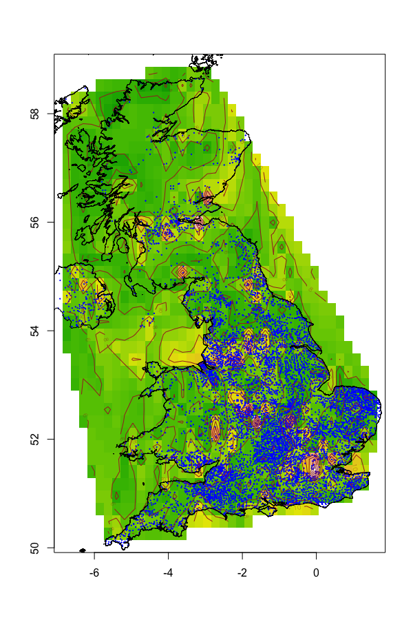
This is a rather naïve plot: interpolation is not aware of water, so interpolates between Stranraer and Belfast regardless of the Irish Sea in the way; however, it looks reasonable on land, with higher values over large centres of population such as London, the Midlands, and the central belt in Scotland (from Edinburgh to Stirling to Glasgow).
The script attempts to train a RandomForest model to look for patterns correlating population with latitude and longitude, outputting the importance of both variables:
> print(importance(model_rf))
          IncNodePurity
latitude   1.516258e+15
longitude  2.375570e+15
It also prints the correlation matrix:
                   latitude      longitude    population
latitude        1.000000000   -0.291285847   0.008083111
longitude      -0.291285847    1.000000000  -0.004161835
population      0.008083111   -0.004161835   1.000000000
Between them, these show there’s some slight relationship between longitude and population, with the contribution from latitude being half as significant. A graph of population vs longitude shows a distinct hump around the middle, effectively projecting London, Edinburgh, Stirling, Glasgow, North(-East) England, and the Midlands, all onto a line, with the less-populated Western Isles, West Country, and Northern Ireland to the left.
Next Steps
Updates
The script above has been updated from previous versions to illustrate updating an RDF triplestore by SPARUL, a/k/a SPARQL Update.
At the core, we define the function df2n3() which unrolls a data.frame to n3 format — simply, every row is treated as an instance of an entity (identified by a subject URI which may optionally be specified in the first column or the entity URI will be minted automatically); column names become predicates (either URI or CURIE), and cell values become triple values. (This reshaping is similar to other relational-to-RDF converters such as our R2RML and Sponger Cartridge for CSV implementations.)
This ntriples string forms the bulk of a SPARUL INSERT DATA statement:
updatequery <- paste("INSERT INTO <urn:temp:rdata> {", n3str, "}")
ret <- SPARQL("http://dba:dba@localhost:8889/sparql", query=updatequery)
SPARQL already allows direct loading from existing URIs with the SPARQL LOAD construct; this function, however, allows transformation of the data using regular R data.frame manipulation functions while the data is in transit.
Federation
SPARQL has a SERVICE keyword that allows federation, i.e., execution of queries against multiple SPARQL endpoints, joining disparate data by common variables (Federated SPARQL a/k/a SPARQL-FED). For example, it should be possible to enrich the data by blending Geonames and the Ordnance Survey gazetteer in the query.
Over to you to explore the data some more!